Accepted by ICLR 2026 Workshop on Scaling Post-training for LLMs!
TL;DR
We present A-3PO (APproximated Proximal Policy Optimization), a method that eliminates the expensive forward pass required by decoupled PPO in asynchronous RL training. By approximating the proximal policy through staleness-aware interpolation instead of explicit computation, we achieve:
- 1.8× speedup in training time (up to 26.15 hours → 14.54 hours)
- 8,500× faster proximal policy computation (10 seconds → 0.001 seconds)
- Better stability with more controlled importance weights
- Comparable or better performance across multiple benchmarks
Code available: Open-source implementation in the AReaL framework
The Problem: Decoupled PPO is Slow
Why Asynchronous RL?
Standard PPO follows a rollout-then-training loop: collect data, then train. This sequential pattern wastes computational resources—GPUs sit idle during rollout, and inference engines sit idle during training.
Asynchronous RL solves this by running rollout and training as parallel engines. This achieves better resource utilization and higher throughput. However, it introduces staleness: the training engine’s target policy can be several updates ahead of the rollout engine’s behavior policy.
The Decoupled Loss Solution
Standard PPO becomes unstable under high staleness because it uses the same old policy $\pi_{\text{old}}$ for two different purposes:
- Importance sampling to correct for off-policy data
- Trust region constraint to prevent destructive updates
Decoupled PPO separates these roles:
$$ \begin{aligned} J(\theta) = \mathbb{E}\Big[\underbrace{\frac{\pi_{\mathrm{prox}}(a_t|s_t)}{\pi_{\mathrm{behav}}(a_t|s_t)}}_{\text{Importance Weight}}\min( \frac{\pi _\theta (a_t|s_t)}{\pi _{\mathrm{prox}}(a_t|s_t)} \hat{A}_t, \mathrm{clip}( \underbrace{\frac{\pi _\theta (a_t|s_t)}{\pi _{\mathrm{prox}}(a_t|s_t)}} _{\text{Trust Region Anchor}}, 1-\epsilon, 1+\epsilon ) \hat{A}_t ) \Big] \end{aligned} $$
Where:
- $\pi_{\mathrm{behav}}$: actual behavior policy that generated the data (for importance weights)
- $\pi_{\mathrm{prox}}$: recent proximal policy (for trust region anchor)
- $\pi_\theta$: current target policy being optimized
This improves stability by anchoring updates to a fresher policy. But there’s a catch: computing $\pi_{\mathrm{prox}}$ requires an extra forward pass through the model at each training step—about 10 seconds for large language models!
The Key Insight
Do we really need to compute $\pi_{\mathrm{prox}}$ explicitly?
Looking at the objective from first principles: the proximal policy simply serves as a trust region anchor. It doesn’t need precise values from the neural network—it just needs to lie somewhere between the behavior and target policies to prevent extreme importance weights.
This leads to our solution: approximate $\pi_{\mathrm{prox}}$ through interpolation.
A-3PO: Staleness-Aware Approximation
The Core Idea
Instead of computing $\pi_{\mathrm{prox}}$ via forward pass, we interpolate it in log-probability space:
$$\log \pi_{\mathrm{prox}} = \alpha\log \pi_{\mathrm{behav}} + (1-\alpha) \log \pi_\theta$$
where $\alpha$ is a staleness-aware coefficient:
$$ \begin{aligned} d &= v(\pi_{\theta}) - v(\pi_{\mathrm{behav}}) \newline \alpha &= \begin{cases} 0, & d = 0 \quad \text{on-policy} \newline \dfrac{1}{d}, & d \ge 1 \quad \text{off-policy} \end{cases} \end{aligned} $$
Here $d$ is the staleness (training step difference), and $v(\pi)$ denotes the policy version.
Why This Works
When on-policy ($d=0$): $\alpha=0$, so $\pi_{\mathrm{prox}} = \pi_\theta = \pi_{\mathrm{behav}}$. This recovers standard PPO.
When off-policy ($d \geq 1$): As staleness increases, $\alpha$ decreases, making $\pi_{\mathrm{prox}}$ closer to the target policy $\pi_\theta$ (the fresher policy) and giving less weight to the stale behavior policy.
This is intuitive: when data is very stale, we trust the current policy more for anchoring the trust region.
Theoretical Guarantees
Our approximation has nice properties:
1. Sandwich Property — $\pi_{\mathrm{prox}}$ stays bounded between the behavior and target policies:
$$\min\{\pi_{\mathrm{behav}}(a | s), \pi_\theta(a | s)\} \le \pi_{\mathrm{prox}}(a | s) \le \max\{\pi_{\mathrm{behav}}(a | s), \pi_\theta(a | s)\}$$
2. Contractive Stability — The importance ratio simplifies to:
$$r(a | s) = \left(\frac{\pi_{\theta}(a | s)}{\pi_{\mathrm{behav}}(a | s)}\right)^{\alpha}$$
As staleness increases ($\alpha \to 0$), importance weights contract toward 1, preventing extreme ratios. Moreover, raising importance weights to power $\alpha < 1$ provably reduces their variance, leading to more stable updates.
Implementation: Remarkably Simple
Here’s the core implementation in PyTorch:
def compute_prox_logp_approximation(
    old_logp: torch.Tensor,      # log π_behav
    logprobs: torch.Tensor,      # log π_θ
    versions: torch.Tensor,      # v(π_behav) per token
    current_version: int,        # v(π_θ)
) -> torch.Tensor:
    """Approximate proximal policy log-probabilities."""
    # Compute staleness: d = v(π_θ) - v(π_behav)
    staleness = float(current_version) - versions.float()

    # Compute staleness-aware coefficient α
    alpha = torch.where(
        staleness >= 1,
        1.0 / staleness,
        torch.zeros_like(versions.float()),
    )

    # Log-linear interpolation
    prox_logp = alpha * old_logp + (1 - alpha) * logprobs

    return prox_logp
That’s it! No neural network forward pass—just element-wise arithmetic on tensors already available in the training loop.
Experiments: Does It Actually Work?
We evaluated A-3PO on mathematical reasoning tasks using the AReaL framework across two setups:
Setup 1: Qwen2.5-1.5B-Instruct on GSM8K
- Model: 1.5B parameter instruction-tuned model
- Dataset: GSM8K (8.5K grade school math problems)
- Baselines: Sync GRPO, Decoupled PPO with recompute
Setup 2: Qwen3-8B on DAPO-Math-17k
- Model: 8B parameter base model
- Dataset: DAPO-Math-17k (17K math problems)
- Baselines: Same as Setup 1
Results: Speed + Stability + Performance
1. Computational Efficiency
Proximal policy computation time:
- Recompute method: ~10 seconds per training step
- A-3PO (loglinear): ~0.001 seconds per training step
- Speedup: 8,500× in proximal policy computation
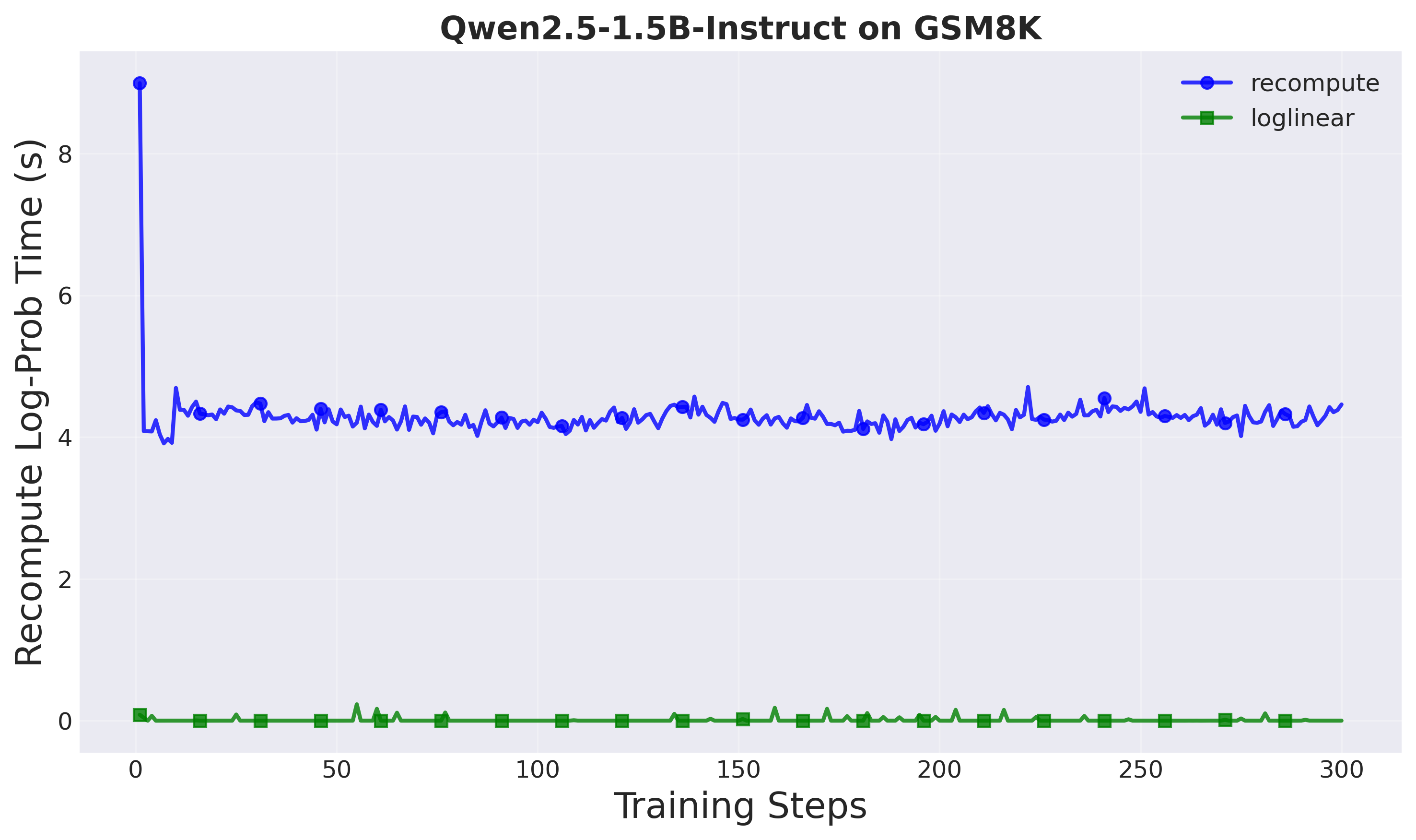
Figure 1: Log probability computation time comparison (Setup 1: Qwen2.5-1.5B). The loglinear method achieves near-instantaneous computation.
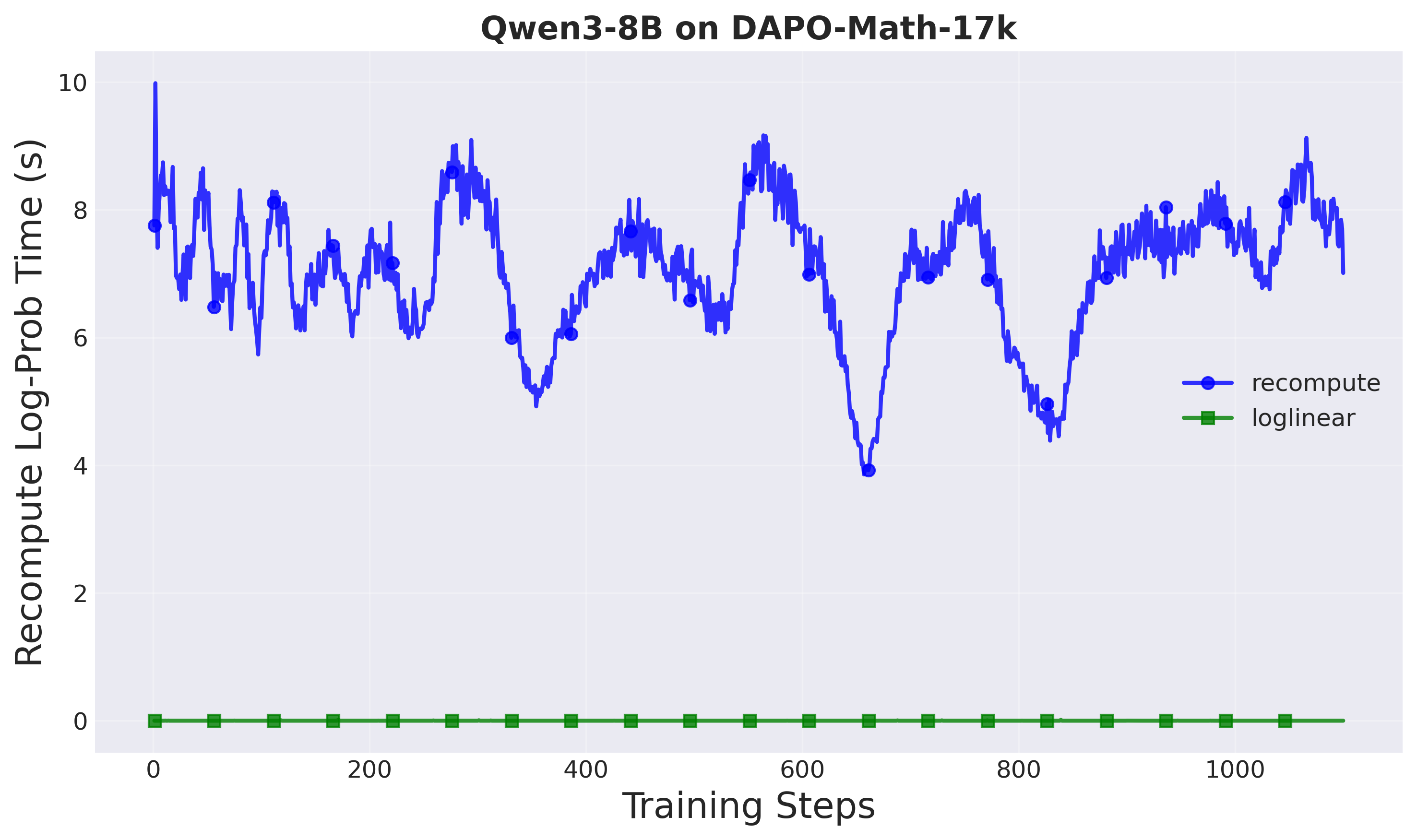
Figure 2: Log probability computation time comparison (Setup 2: Qwen3-8B). The 10-second forward pass overhead is eliminated.
Overall training time:
| Setup | Method | Training Time | Speedup |
|---|---|---|---|
| Setup 1 (1.5B) | Sync GRPO | 2.36 hours | — |
| Recompute | 1.82 hours | 1.3× | |
| A-3PO | 1.53 hours | 1.5× | |
| Setup 2 (8B) | Sync GRPO | 26.15 hours | — |
| Recompute | 16.10 hours | 1.6× | |
| A-3PO | 14.54 hours | 1.8× |
The speedup is more pronounced at larger model scales, where forward passes are more expensive.
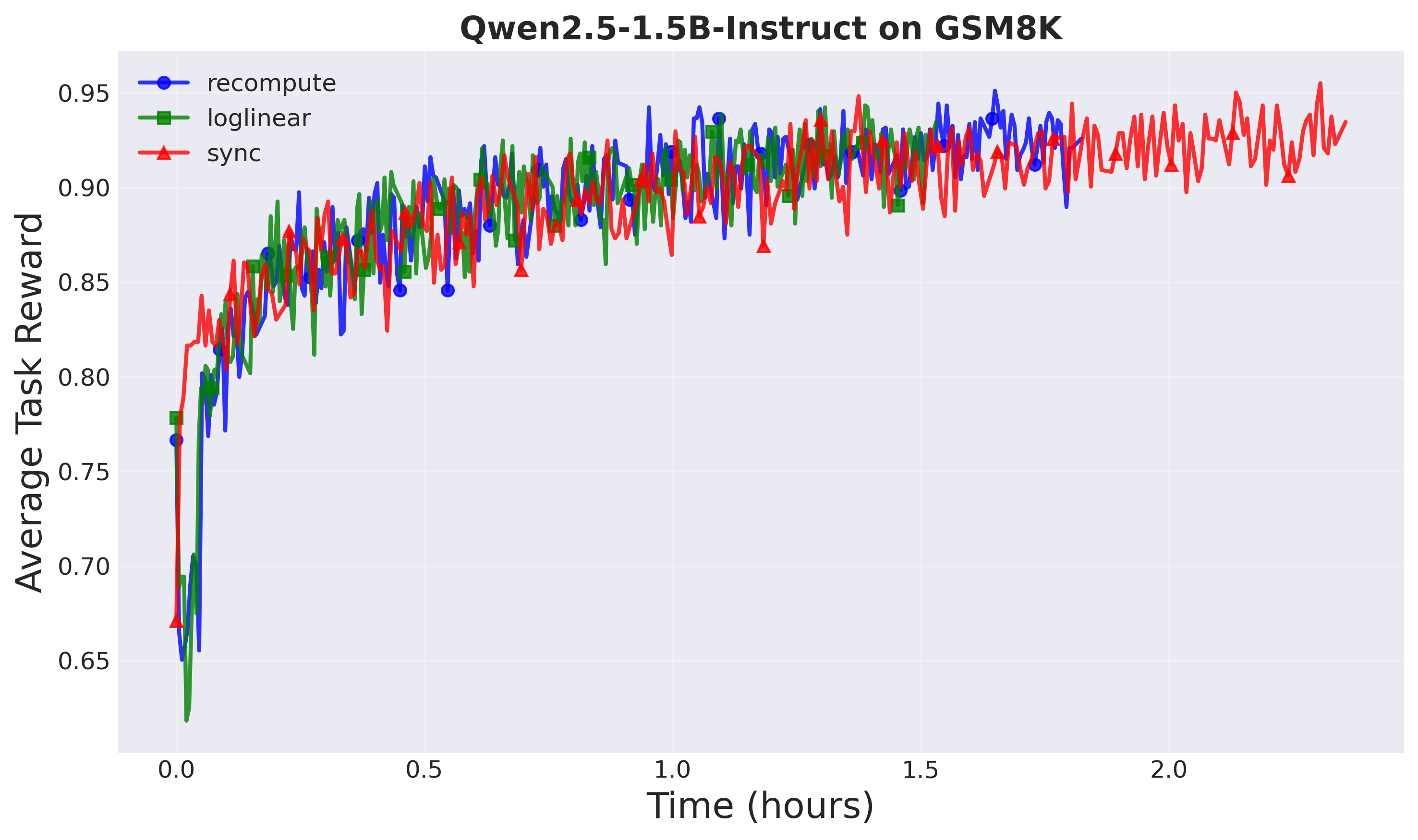
Figure 3: Training progress (Setup 1: Qwen2.5-1.5B). A-3PO reaches the same reward faster.
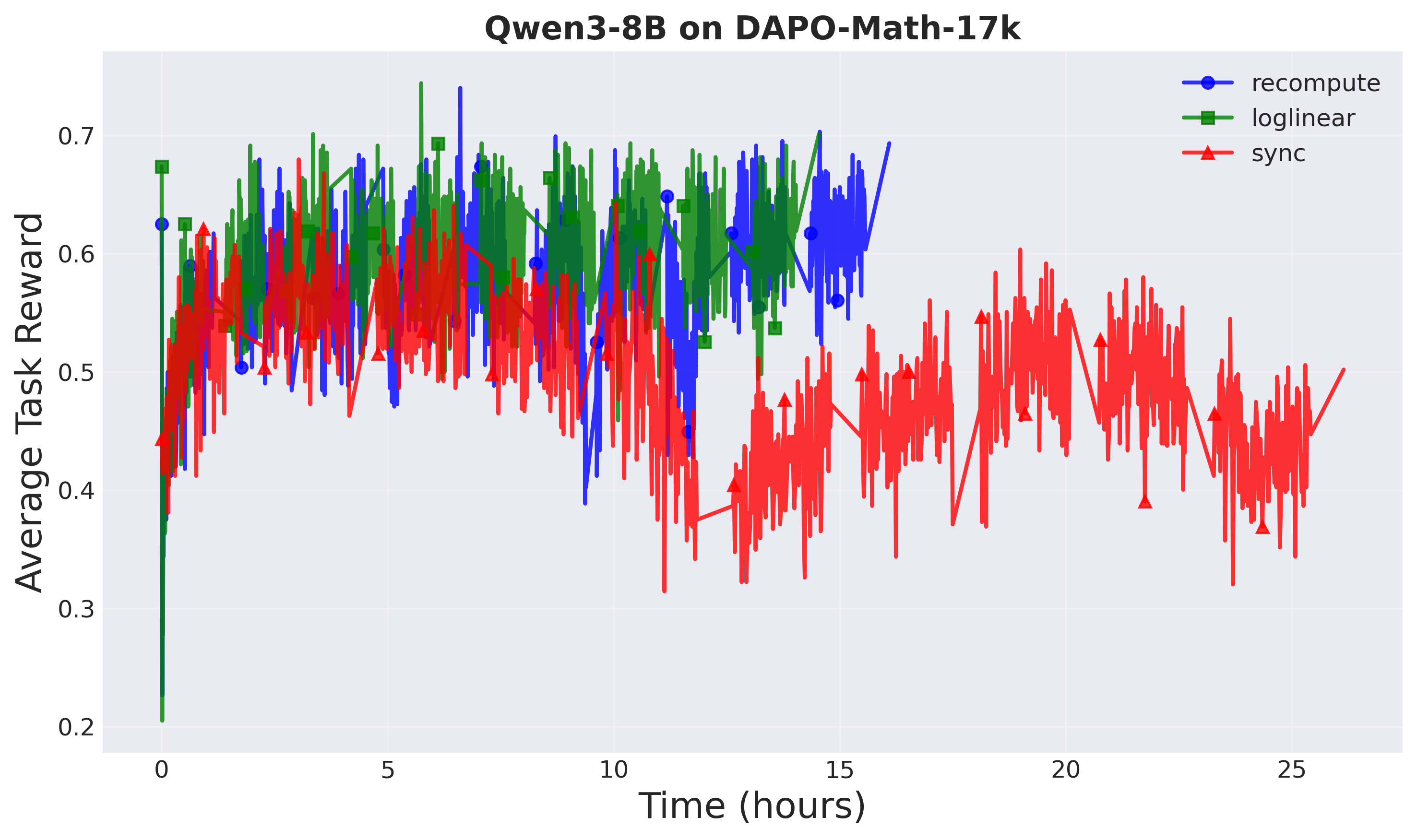
Figure 4: Training progress (Setup 2: Qwen3-8B). Asynchronous training with A-3PO achieves 1.8× speedup.
2. Task Performance
Final evaluation rewards:
| Setup | Method | Eval Reward |
|---|---|---|
| Setup 1 | Sync GRPO | 0.793 |
| Recompute | 0.797 | |
| A-3PO | 0.791 | |
| Setup 2 | Sync GRPO | 0.443 |
| Recompute | 0.627 | |
| A-3PO | 0.623 |
A-3PO maintains comparable performance to recompute while being significantly faster. Notably, both async methods (recompute and A-3PO) substantially outperform sync GRPO in Setup 2, demonstrating the effectiveness of decoupled loss at larger scales.
Benchmark evaluation on AIME24 and MATH500 (Setup 2):
| Method | AIME24 pass@1 | MATH500 pass@1 | Average |
|---|---|---|---|
| Sync GRPO | 40.00 ± 9.10% | 46.80 ± 2.23% | 43.40% |
| Recompute | 66.67 ± 8.75% | 62.80 ± 2.16% | 64.74% |
| A-3PO | 66.67 ± 8.75% | 66.60 ± 2.11% | 66.64% |
A-3PO achieves the best performance on challenging mathematical reasoning benchmarks while being the fastest method.
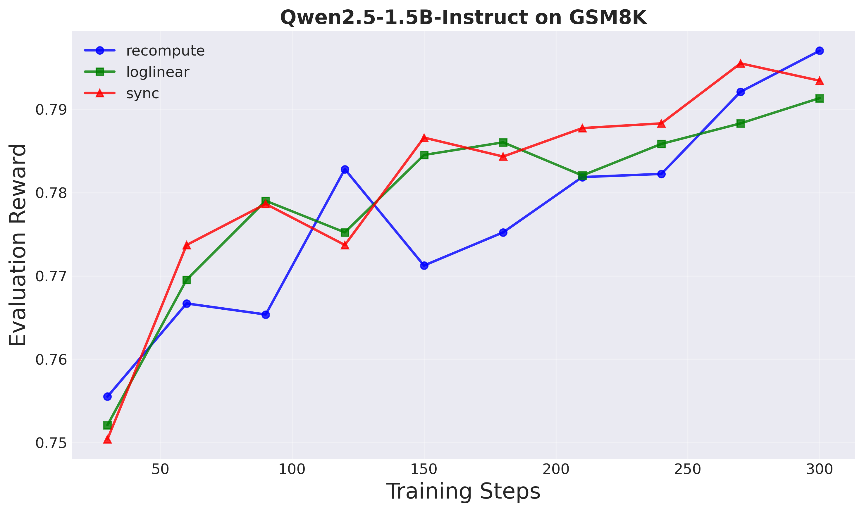
Figure 5: Evaluation reward on held-out test prompts (Setup 1). All methods converge similarly.
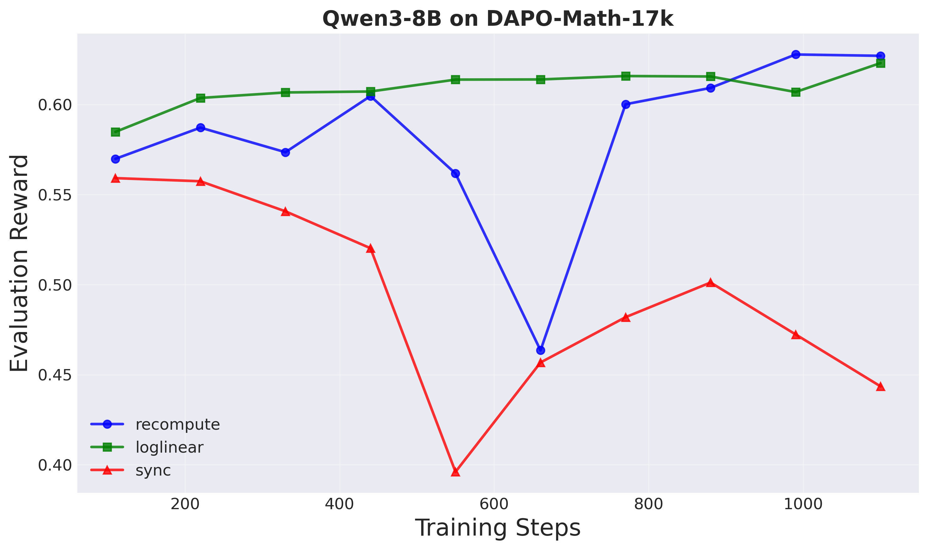
Figure 6: Evaluation reward on held-out test prompts (Setup 2). Asynchronous methods substantially outperform sync.
3. Training Stability
Importance weights: A-3PO shows more controlled importance weights compared to recompute, especially at larger scales. In Setup 2, recompute exhibits very high importance weights (indicating instability), while A-3PO maintains stable behavior.
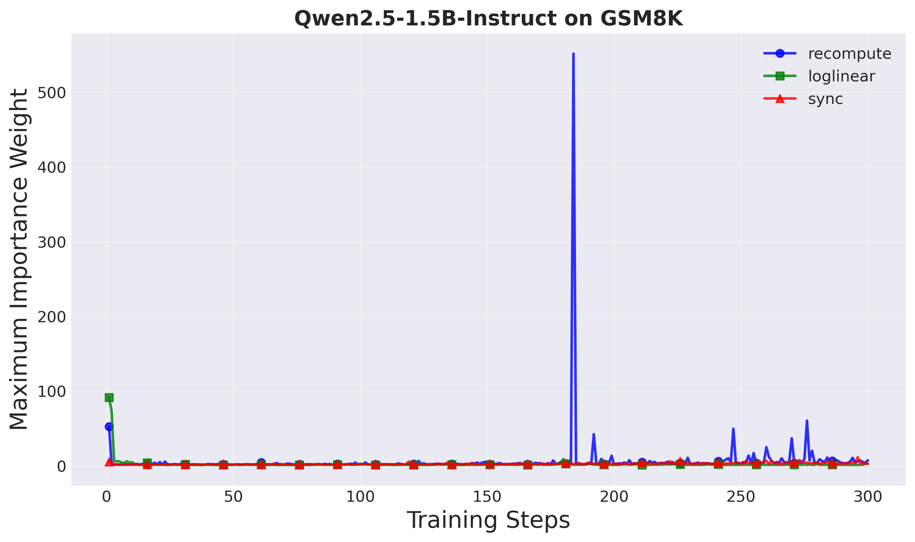
Figure 7: Maximum importance weights (Setup 1). Loglinear shows more controlled weights.
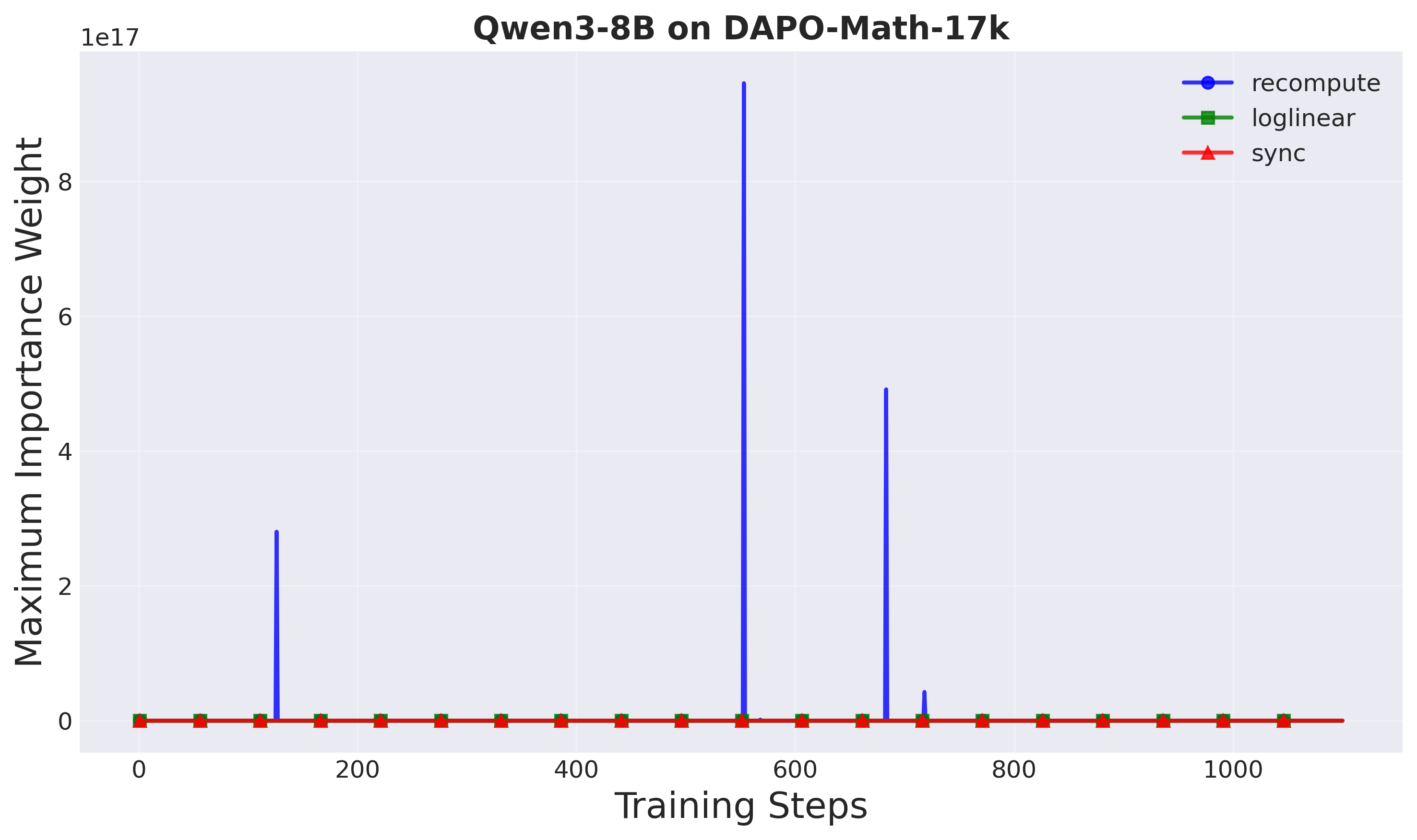
Figure 8: Maximum importance weights (Setup 2). Recompute produces very high weights, indicating instability at larger scales.
Clipped tokens: A-3PO clips the fewest tokens across both setups, suggesting smoother policy updates that naturally stay within trust region bounds. Fewer clipped tokens means:
- More sample-efficient learning
- Less wasted computation on rejected gradients
- Better utilization of collected data
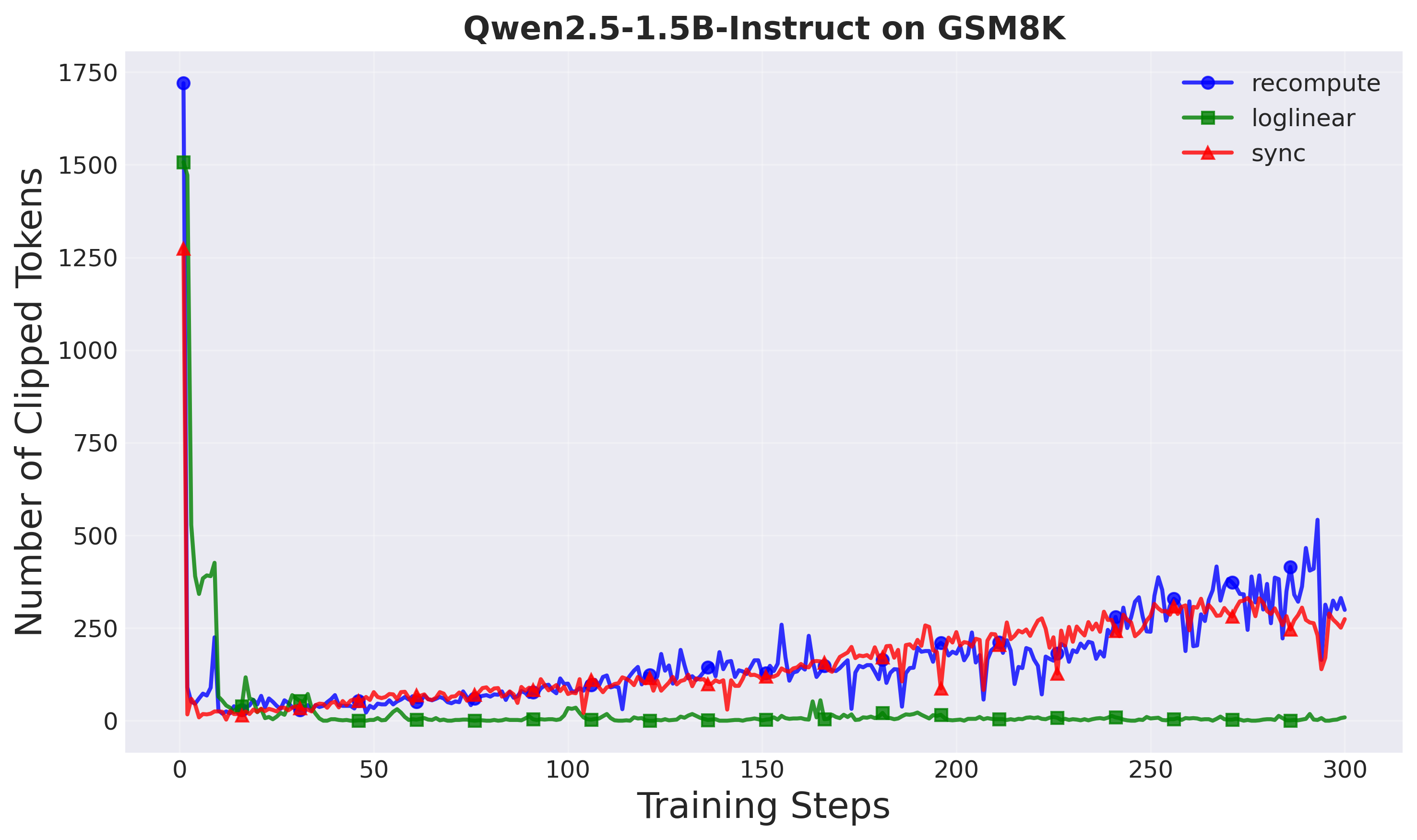
Figure 9: Number of clipped tokens per training step (Setup 1). Loglinear clips the least.
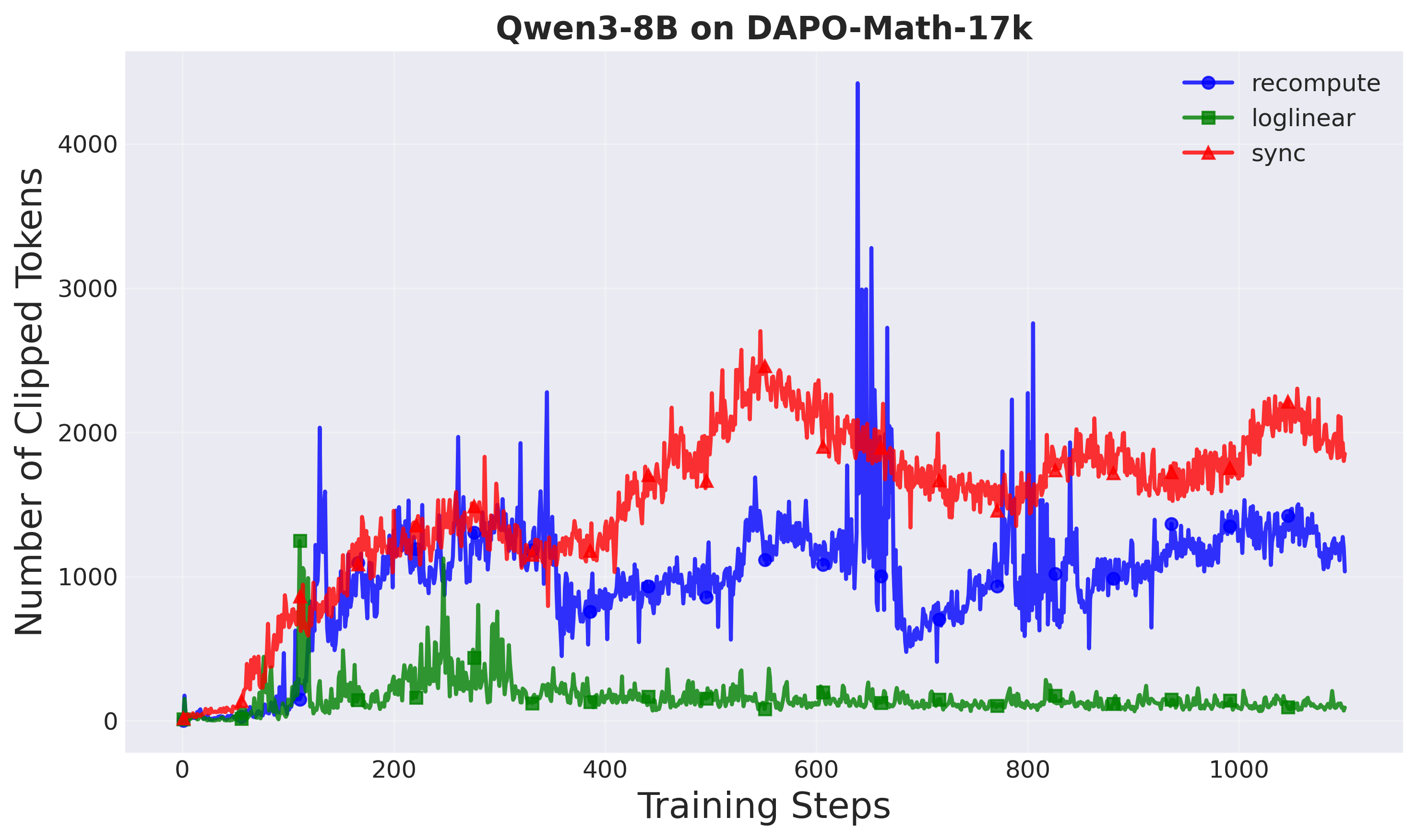
Figure 10: Number of clipped tokens per training step (Setup 2). Fewer clipped tokens indicate better sample efficiency.
Policy entropy: All methods show healthy entropy decay patterns, indicating stable exploration dynamics.
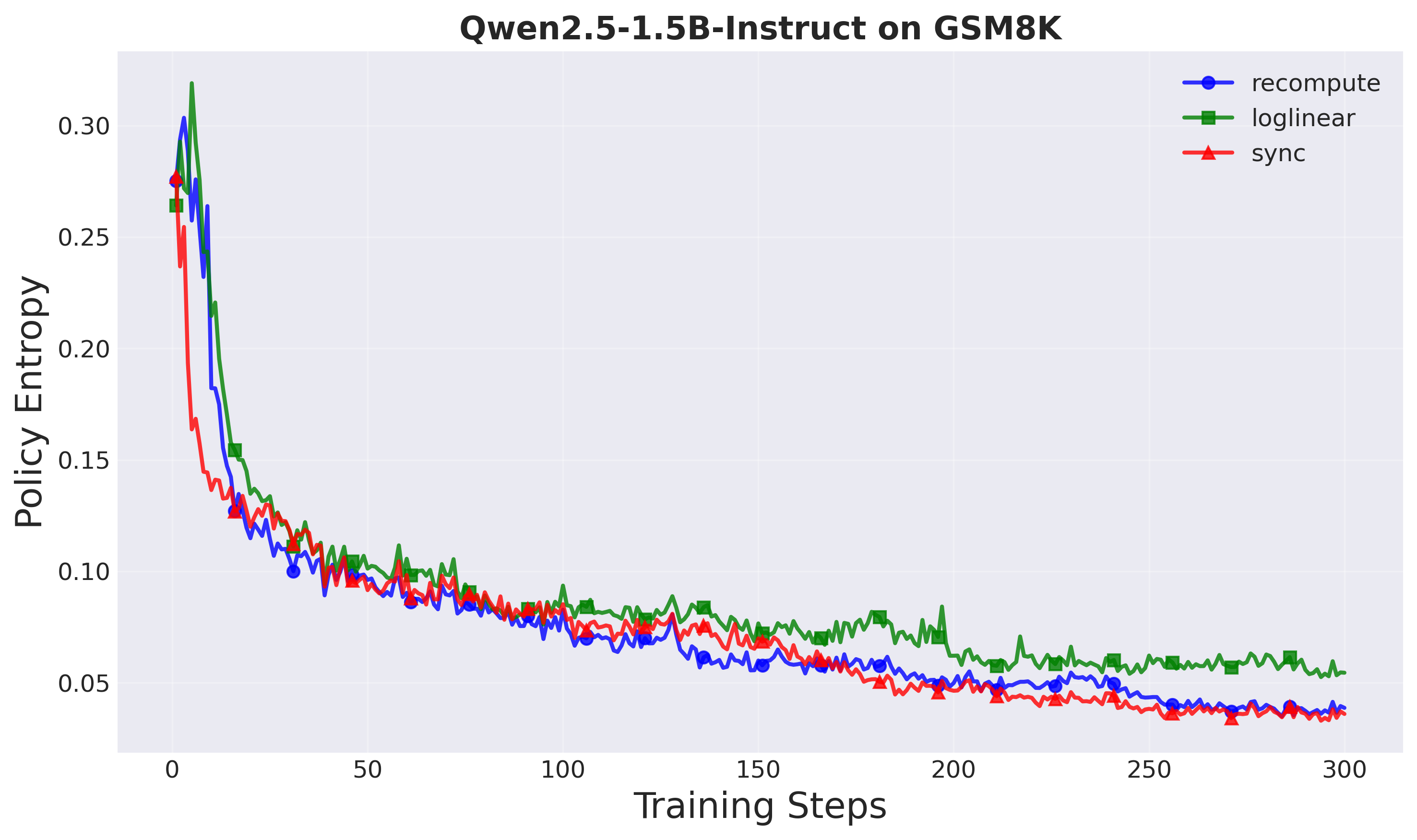
Figure 11: Policy entropy over training steps (Setup 1). Healthy entropy decay for all methods.
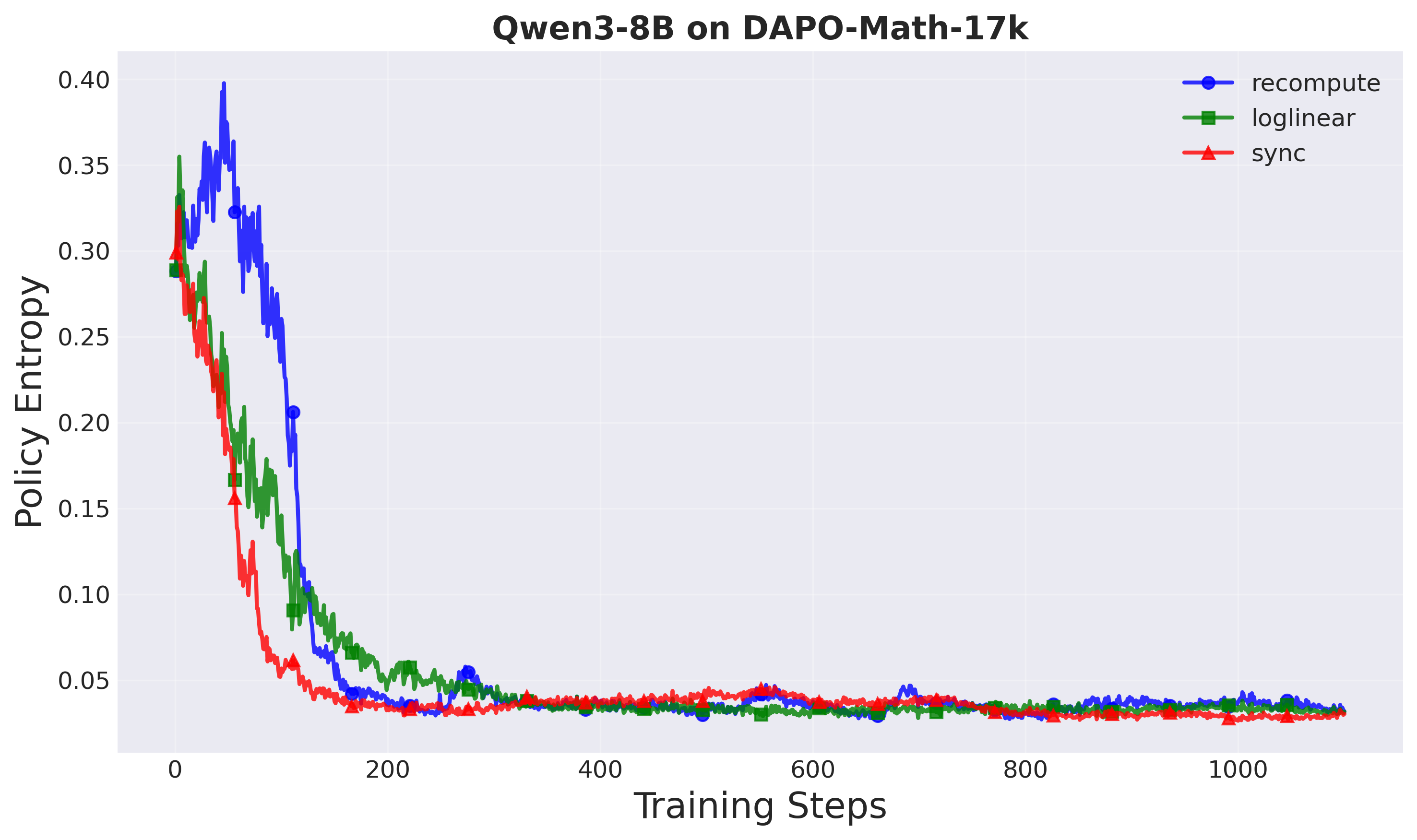
Figure 12: Policy entropy over training steps (Setup 2). All methods show stable exploration dynamics.
Why Does Approximation Work Better Than Exact Computation?
This is a fascinating result: the approximation is not just faster but also more stable than explicit computation. Why?
Our hypothesis: At larger model scales, the recomputed proximal policy may introduce noise or instability due to:
- Numerical precision issues with very small probabilities
- Gradient artifacts from detaching the proximal policy
- Inconsistencies in batch normalization or dropout layers
By contrast, interpolation in log-space is numerically stable and guarantees smooth transitions between policies through the contractive property $r(a|s) = w(a|s)^\alpha$.
This suggests a broader principle: simpler can be better. When designing algorithms for large-scale systems, we should question which components truly require expensive computation and which can be approximated from first principles.
Practical Implications
For Practitioners
If you’re training LLMs with asynchronous RL:
- Use A-3PO instead of explicit proximal policy computation—it’s a simple drop-in replacement
- Expect larger speedups at larger model scales (1.5× at 1.5B → 1.8× at 8B)
- Monitor importance weights as a stability indicator
For Researchers
This work opens several directions:
- Other staleness-aware coefficients: We used $\alpha = 1/d$, but other functions could work
- Extension to other algorithms: The approximation principle applies to any decoupled policy optimization method, not just PPO
- Theoretical analysis: Tighter bounds on approximation error and convergence properties
Conclusion
Decoupled PPO made asynchronous RL stable but slow. A-3PO makes it stable AND fast by recognizing that the proximal policy doesn’t need expensive neural network evaluation—it just needs to lie between the behavior and target policies.
Key takeaways:
- 8,500× faster proximal policy computation
- 1.8× overall training speedup at 8B scale
- Better stability with controlled importance weights
- Best benchmark performance among all methods
The insight is simple: when designing RL algorithms for large-scale systems, question which components truly require expensive computation.
Code & Resources
- Open-source implementation: Available in the AReaL framework
Try A-3PO in your asynchronous RL training and see the speedup for yourself!
References
If you found this work useful, consider citing:
@misc{li2026a3poacceleratingasynchronousllm,
      title={A-3PO: Accelerating Asynchronous LLM Training with Staleness-aware Proximal Policy Approximation},
      author={Xiaocan Li and Shiliang Wu and Zheng Shen},
      year={2026},
      eprint={2512.06547},
      archivePrefix={arXiv},
      primaryClass={cs.LG},
      url={https://arxiv.org/abs/2512.06547},
}
Questions or comments? Feel free to reach out or open an issue on the GitHub repository!